Main Contact
Jaclyn A. Card, Ph.D., Professor
Department of Parks, Recreation and Tourism
University of Missouri
105 Anheuser-Busch Natural Resources Building
Columbia, MO 65211
(573) 882-9516
cardj@missouri.edu

The study examined the relationship between the spatial distribution of public lands used for outdoor recreation and the racial and socioeconomic characteristics of local residents. Specifically, the researchers analyzed demographic characteristics of census block groups within close proximity to outdoor state and national parks in Missouri. Findings implied that whites with low income and blue collar occupations are more likely to live close to the parks than other groups.  The spatial patterns indicated that the demographic makeup of residents is spatially associated with the geographic distribution of outdoor recreation lands. Outdoor recreation planners can use the results when planning new areas or enhancing existing areas by considering the makeup of the surrounding community.

Key Words: spatial relationship, GIS, outdoor recreation, state parks, national parks.

With the issuance of Executive Order 12898 in 1994, federal land management agencies were directed to develop agency-wide environmental equity strategies and to identify patterns of natural resource use among minority and low income populations (Cutter, 1995). Literature published since the enactment of the Executive Order focuses mainly on the distributional impacts of locally unwanted land uses (LULUs) such as the relationship between socioeconomic factors and the location of hazardous facilities. For example, some studies indicated that communities comprising low-income and minority residents were located closer to LULUs than communities comprising high-income and white residents (Bryant, 1995; Hamilton, 1995; Kriesel, Centner, & Keeler, 1996). Also, racial minorities and low-income groups typically had greater exposure to environmental hazards than racial majorities and affluent groups (Bullard, 1994; EPA, 1997; Mohai & Bryant, 1992).

In the field of outdoor recreation, spatial relationship research is in its infancy. Though the Executive Order was issued a decade ago, few studies have addressed outdoor recreation patterns on federal lands (Porter & Tarrant, 2001; Tarrant & Cordell, 1999).  The limited research that does exist indicates that lower income households were more likely to be located within one mile of a wilderness area, campground or fisheries habitat than those with higher incomes (Tarrant & Cordell). A subsequent study of federal sites in Southern Appalachia (Porter & Tarrant) indicated that predominantly white residents with blue-collar occupations and low income lived near national forests and national recreation areas. They concluded that socioeconomic groups and demographic factors may play a role in the spatial distribution of outdoor recreation areas.

Previous research has indicated that ethnic minorities and low income populations bear a disproportionate share of environmental risks due to racial discrimination. Bullard (1983) found that the geographic distribution of minorities and low income populations were disproportionately located close to solid waste sites.  In 1994, Bullard expanded his work and discovered that these populations were exploited not only in the placement of land fills but also in the location of toxic waste dumps.  Mohai and Bryant (1992) agreed with Bullard’s findings; however, he concluded that race has an impact on the distribution of environmental hazards independent of income.  Other researchers suggested that differential exposure to environmental risk may occur for reasons not related to discrimination against any demographic group.  For instance, lack of political power (Hamilton, 1995) or house values, presence of an interstate highway, and population density (Kriesel, et al., 1996) were better predictors of waste sites. Researchers agree, however, that inequities exist, whether racial, socioeconomic or political.  Over time, research has broadened to include occupation status, recreation on public lands, and the sustainability of local communities (Floyd & Johnson, 2002; Tarrant & Cordell, 1999).  Floyd and Johnson provided an in-depth discussion of these issues and concluded that “[R]esearch of this kind is critical for establishing inequitable outcomes [and] documenting spatial relationships between unwanted or undesirable land uses and demographic groups” (p. 72).

Following the lead of Floyd and Johnson (2002), this study provided a spatial pattern on which to build a conceptual basis of how outdoor recreation lands are spatially associated with the specific demographic composition of local residents. This study extended previous work by expanding the spatial relationships between three demographic groups and specific types of outdoor recreation uses at three distances.

Census block groups (CBGs) are a cluster of the smallest geographic area for which census data are gathered.  CBGs represent a collection of census blocks within a census tract, containing 250 to 550 housing units (U.S. Census Bureau, 2002). Specifically, the study analyzed the demographic characteristics of CBGs within one-mile, five-miles, and ten-miles of outdoor recreation areas, and examined the spatial relationship of the specific outdoor recreation land uses to the demographic makeup of proximate CBGs.  This study tested the following hypothesis:  Race, occupation, and household income are significant variables for explaining the geographic distribution of outdoor recreation areas.

Research Design and Data Source
Secondary data was obtained from the 2000 Census Summary File 3 and Missouri public lands data (CARES, 2002). Characteristics of CBGs within a one-mile, five-mile, and ten-mile radius of outdoor recreation public lands in Missouri were identified and the spatial relationships of outdoor recreation areas to the demographic factors of local communities were examined.

A complete count census was used because it provides a CBG, the smallest geographic unit.  Census 2000 Summary File 3 contains CBGs with information about population, income and occupation. CBGs are small units that mirror neighborhood effects because they are smaller than zip code areas, counties and cities (Kriesel, et al., 1996).  Data were downloaded to shapefiles from the CARES website (www.cares.missouri.edu) and FTP site (ftp://www.cares.missouri.edu/pub).

Three demographic variables were analyzed: race (white and nonwhite), median household income, and occupation (white collar and blue collar). Variables were retrieved from the 2000 CBG database from TIGER (Topologically Integrated Geographic Encoding and Referencing) compiled by the Bureau of the Census and maintained by CARES.

Missouri public lands managed by Missouri State Parks (MSP) and the National Park Service (NPS) were the data sources used in the study. An MSP planner classified MSP land into four categories according to their primary attraction: water-based state parks (n=30), historical state parks (n=33), nature-based state parks (n=26) and day-use state parks (n=21).  Water-based parks contained lake or river recreation areas; historic parks concentrated on preserving and interpreting historical and cultural resources; nature-based parks were those other than water and historical parks with overnight camping; and day-use parks included types of activities such as picnicking and hiking with no overnight camping.  The researchers used the National Park Service use designations for NPS areas.  There were nine water-based and four historical designations.

Spatial Analysis
GIS is a recent methodology in outdoor recreation and few researchers have conducted studies using GIS; yet GIS is a flexible and effective decision support tool in land use planning (Feick & Hall, 2000).  Feick and Hall applied GIS-based decision support for consensus building and conflict identification in tourism development planning. Other studies suggested using GIS for marketing and recreational and park management (Nedovic-Budic, Knaap, & Scheidecker, 1999; Nicholls & Shafer, 2001).  Tarrant and Cordell (1999) used GIS to examine the spatial distribution of outdoor recreation sites and their relationship to communities. Similarly, Porter and Tarrant (2001) used GIS to examine the federal lands covering 135 counties in Southern Appalachia.

Following previous research (Feick & Hall, 2000; Porter & Tarrant, 2001; Tarrant & Cordell, 1999), this study used Arcview GIS version 3.2 and created a new map by adding the shapefile of the Missouri public lands and the shapefile of CBGs.  A shapefile is a digital file consisting of one layer of mapped geographic information. The shapefile of Missouri public lands contains information on all the exact geographic locations, areas, perimeters, land users, management systems, land names, and land owners. The shapefile of CBGs includes information on geographic location and demographic information such as race, income, and occupation.

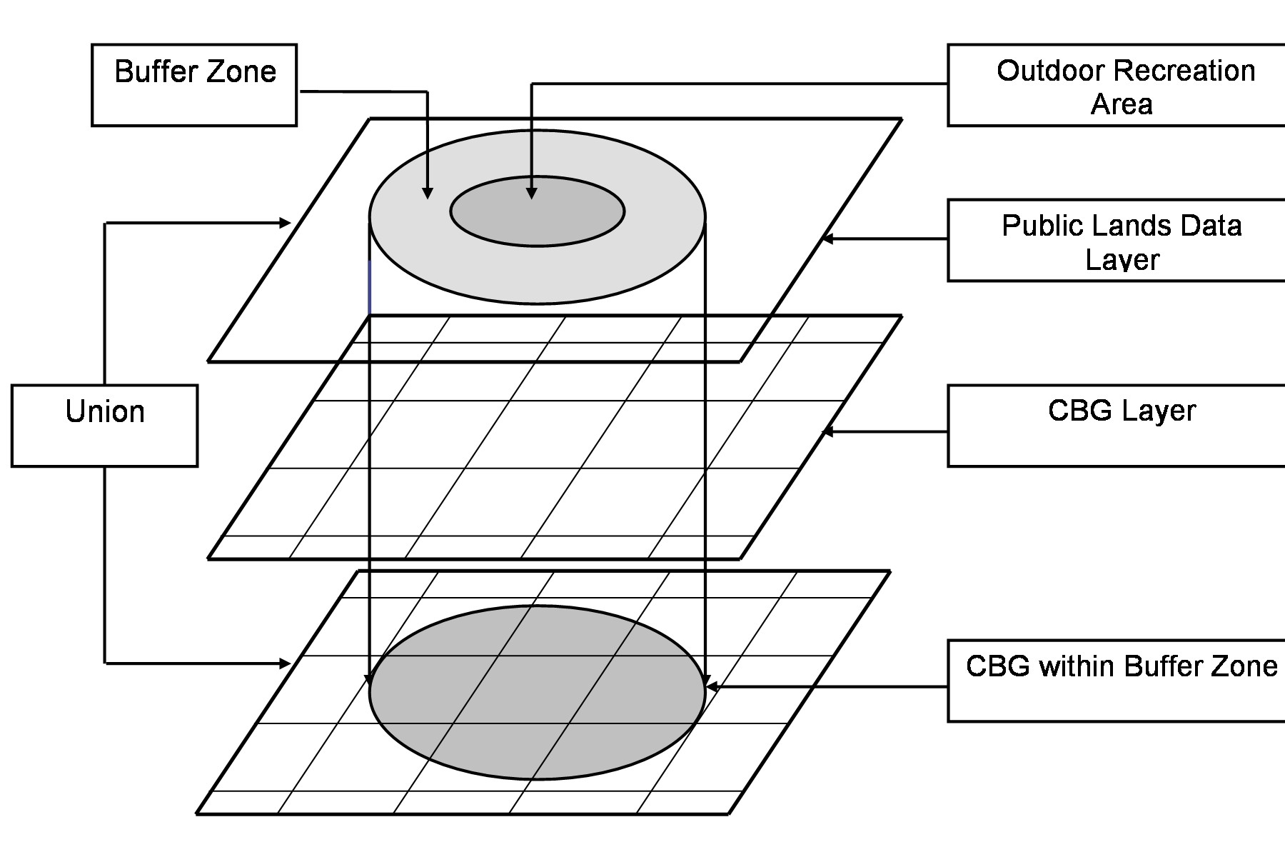
Using Query Builder, the researchers selected relevant public lands datasets according to the classified categories. Next, the selected datasets were converted to shapefiles to create a new shapefile specific to the study. The new shapefiles represented the six types of outdoor recreation areas.  The relevant outdoor recreation areas were buffered with specific distances to separate the CBGs in close proximity to these areas from CBGs outside the distances. Using GeoProcessing Wizard within ArcView, the geometry and attributes of public land data shapefile and CBG data layers were combined to create a new output using Union, a map overlay method. The output shapefiles generated by Union included attribute information on location and CBG data.  Then Avenue Script within ArcView was used to calculate feature geometry values and update the area and perimeter in the overlay outputs. A percentage of the new area was assigned in the attribute table of the overlay outputs based on the proportion of the new area to the old area. Figure 1 shows the spatial analysis using buffering and Union to identify the CBGs within a buffer zone.

Figure 1

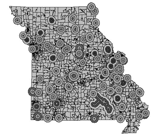
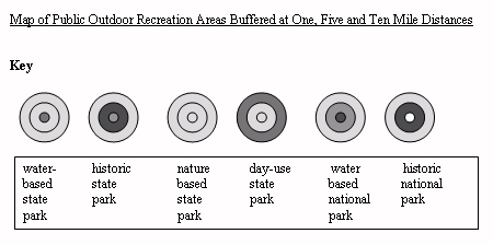
CBGs within buffer zones were coded 1 and those outside buffer zones were coded 0. Any CBG overlapping less than five percent of a buffer zone was coded as outside the boundary, correcting for over-influence by low-population block groups in rural areas.  Query Builder was used to designate buffer zones.  The datasets were then exported to SPSS as database files. Figure 2 depicts the buffer zones for the outdoor recreation areas.

Figure 2

 Consistent with statistical analyses in previous studies (Hamilton, 1995; Porter & Tarrant, 2001; Tarrant & Cordell, 1999), this study used logistic regression to determine the spatial relationships. Logistic regression overcomes restrictive assumptions of ordinary least squares (OLS) regression. It is used when the dependent variable is a dichotomy and the independent variables are continuous, categorical, or mixed because it does not assume linearity of relationship between the dependent and independent variables and it does not require normally distributed variables. Logistic regression calculates changes in the log odds of the dependent variables, not change in the dependent variables itself as does OLS regression. The logistic regression analysis makes comparisons of the probability of an event occurring with the probability of the event not occurring. For each possible set of values for the independent variables, there is a probability that an event occurs. A positive coefficient increases the probability that an event occurs while a negative coefficient decreases the predicted probability (Hair, Anderson, Tatham, & Black, 1992).

Distance was coded 1 if a CBG was within specified distances (one mile, five miles, and ten miles) of recreation sites and coded 0 if a CBG was outside the distances. Race was categorized as white and nonwhite and occupation as white-collar and blue collar.  Income was a continuous variable measured as the median value per household (Porter & Tarrant, 2000).  Independent variables were percentage nonwhite (X1), percentage blue-collar occupation (X2) and median household income in dollars (X3).

To test the hypothesis, the researcher assessed the significance values for the independent variables based on the Wald statistic. The Model Chi-Square was used as an indicator of model appropriateness to determine if the overall model was statistically significant as the goodness-of-fit measure. A significant Chi-square indicates the independent variables together explain variance in the dependent measure. Logistic regression provides two measures that are analogs to R² in OLS regression: Cox and Snell’s R² and Nagelkerke’s R². This study used Nagelkerke R² because it is more stringent than the Cox and Snell’s R² (Hair, et. al, 1992).

Missouri consists of 4,540 CBGs. The area contained a majority of whites (81.64%) which was higher than the national white population (75.1%). Less than half of the sample was composed of blue-collar workers (M = 45.08%; SD=18.36).  The median household income for the entire CBGs (M = $34,808; SD=$21,697) was lower than the national median income of $41,994 (U.S. Bureau of the Census, 2002).

Description of Outdoor Recreation Areas

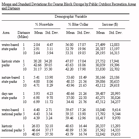
Table 1 shows the means and standard deviations of the three demographic variables for the CBGs surrounding each of the park types based on their distance from the parks. Overall, areas surrounding historic national parks had the highest percentage of nonwhites (M=46.64% at five miles; SD=37.17).  Areas surrounding water-based national parks had the largest percentage of blue collar occupations (M=59.67% at one mile; SD=17.26) and the lowest income (M=$17,792 at five miles; SD=$9,544). Those surrounding water-based state parks had the lowest percentage of whites (M=2.84% at one mile; SD=4.47), the lowest percentage of blue collar occupations (M=34.41% at ten miles; SD=21.76) while the highest income (M=$47,512 at ten miles; SD=$34,257) was in areas surrounding day-use state park areas.  Only areas surrounding historic state parks and historic national parks had populations greater than 25% nonwhite.  All areas had over one-third blue collar occupations, while income varied widely from the high teens to the mid-forties.  Twelve areas had lower percent nonwhite and lower income than Missouri overall and five had fewer blue-collar workers.

Table 1

Logistic Regression Analysis for Each Type of Outdoor Recreation Area
Table 2 shows the logistic regression coefficients and the Chi-square statistics of the CBGs in close proximity to the study areas. The results supported the hypothesis that the three demographic variables (race, occupation, household income) were significant independent variables for explaining the communities’ proximity to the outdoor recreation areas.  Of the three independent variables, nonwhite and income retained the most significant and consistent coefficient signs while the coefficients for blue-collar occupations retained inconsistent signs.

Table 2

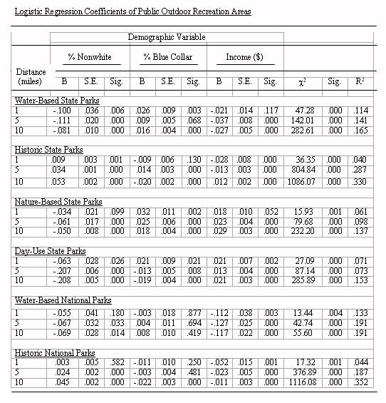
Water-Based State Parks
The overall model fit for areas surrounding water-based state parks was statistically significant (p<.05). Percent nonwhite was significant (p<.05) at all three distances and negatively related to the distribution of these areas. Percent blue-collar was significant (p<.05) except for the five-mile distance and positively related to these areas. Median household income was also significant (p<.05) with the exception of CBGs within a one-mile distance. For all three distances, coefficient values on the percentage nonwhite and income were negative and coefficient values on the percentage blue-collar were positive. Findings indicated that a higher percentage of whites with lower incomes and blue-collar occupations resided in close proximity to water-based state parks.

Historic State Parks
Chi-square was statistically significant (p<.05) showing that all three models were a good fit. R²  increased for the model farther away from the areas, suggesting that the model performs better when it covers a wider area of CBGs surrounding historic state parks. Percent nonwhite was significant (p<.05) at all three distances and positively related to the distribution of the areas, indicative of a higher percentage of nonwhites living close to historic state parks. The percent blue-collar was significant (p<.05) except for the CBGs within one mile. The significant coefficient for the percent blue-collar was positive at the five-mile distance and negative at ten miles. Median household income was significant (p<.05) with a negative sign at one-mile and five-mile distances and a positive sign at ten miles. The coefficients on the income and occupation variables changed according to distances. As the income variable moved away from historic state parks, the coefficient for the income changed from negative to positive. CBGs surrounding historic state parks included a higher percentage of nonwhite and low income populations.

Nature-Based State Parks
The overall model fit was statistically significant (p<.05). Percent nonwhite was significant (p<.05) except for one mile and negatively related to the distribution of the areas. Percent blue-collar was significant (p<.05) and positively related to these sites, indicating that blue-collar workers were more likely to be residing near this type of recreation area. Median household income was significant (p<.05) with the exception of the CBGs within one mile distance and positively related to these areas. A higher percentage of white individuals with higher incomes and blue-collar occupations were more likely to live in close proximity to nature-based state parks, suggesting that this type of recreation land is spatially associated with an affluent white population.

Day-Use State Parks
The overall model fit was statistically significant (p<.05). Percent nonwhite was significant (p<.05) at all three distances and negatively related to the distribution of the parks. Percent blue-collar was significant (p<.05) at all distances and negatively related to the sites at five and ten miles. Median household income was significant (p<.05) and positively related to the areas at all distances.  The coefficient values on the percentage nonwhite and blue collar variables were negatively related at five and ten miles and the coefficient value on income was positive at all distances. The findings indicated that white-collar and high income populations reside in close proximity to day-use state parks.

Water-Based National Parks
The overall model fit was statistically significant (p<.05). Percent nonwhite was significant (p<.05) at five-mile and ten-mile distances and negatively related to the distribution of these areas. Occupation variables were not statistically (p>.05) significant regardless of distances. Income was significant (p<.05) and negatively related to the CBGs within all distances. The coefficient values on the percentage nonwhite and income were negative, suggesting that a higher percentage of non-whites with lower incomes resided in close proximity to this type of outdoor recreation land.

Historic National Parks
At all distances, the overall model fit was significant (p<.05). R² increased as distance increased signifying that the three demographic variables explained more variance when they contained a wider area of CBGs surrounding historic national parks. Percent nonwhite was significant (p<.05) with the exception of the one-mile distance and positively related to the distribution of the areas. Percentage blue-collar was only significant (p<.05) at ten miles and negatively related to the areas. Within all distances, income was significant (p<.05) and negatively related to the CBGs near the parks. The coefficient values on the percent nonwhite were positive and the coefficients on the income were negative, signifying that a higher percentage of non-whites with lower incomes were residing near historic national parks.

Previous studies used one-mile distances as the cut-off spatial value (Porter & Tarrant, 2001; Tarrant & Cordell, 1999); this study, however, used one-mile, five-mile, and ten-mile buffer distances.  One mile was the least stable indicator of spatial distribution of public outdoor recreation areas.  Why this difference occurred will require additional studies.

Some communities may perceive outdoor recreation areas as locally undesirable land uses because of their perceived or real negative impacts such as crowding and environmental degradation. Others may think that positive aspects outweigh negative aspects and factors such as aesthetic beauty, clean air, and clean water make outdoor recreation areas a desirable place to live (Porter & Tarrant, 2001). When defining the costs and benefits of outdoor recreation land uses, one must recognize the perspectives of diverse groups living in the immediate areas (Floyd & Johnson, 2002). In addition to determining the spatial relationship, further research should examine how residents perceive specific types of outdoor recreation land use and what actual impacts the land has on local people in both economic and non-economic terms.  Only then will spatial relationship be understood in the context of outdoor recreation.

Bullard, R. D. (1983). Solid waste sites and the black Houston community. Sociological Inquiry, 3, 273-288.

Bullard, R. D. (1994). Decision making. Environment 36, 11-20.

Center for Agricultural, Resource and Environmental Systems. [CARES]. (2002). About CARES. Online document retrieved August 10, 2002 at
          http://www.cares.missouri.edu/cares/about/index.html

Cutter, S. (1995). Race, class and environmental justice. Progress in Human Geography, 19(1), 111-122.

Feick, R. D., & Hall, G. B. (2000). The application of a spatial decision support system to tourism-based land management in small island states. Journal of Travel
          Research, 39, 63-171.

Floyd, M. F., & Johnson, C. Y. (2002). Coming to terms with environmental justice in outdoor  recreation: A conceptual discussion with research implications.
          Leisure Science, 24, 59-77.

Hair, J.F., Anderson, R.E., Tatham, R.L., & Black, W.C. (1992). Multivariate data analysis. New York: Macmillan Publishing Company.

Hamilton, J. T. (1995). Testing for environmental racism: Prejudice, profits, political power?  Journal of Policy and Management, 14, 107-132.

Kriesel, W., Centner, T. J, & Keeler, A. G. (1996). Neighborhood exposure to toxic releases: Are there racial inequities? Growth and Change, 27, 479-499.

Mohai, P., & Bryant, B. (1992). Race and the incidence of environmental hazards: A time for  discourse. Boulder, CO: Westview.

Nedovic-Budic, Z., Knaap, G., & Scheidecker, B. (1999). Advancing the use of geographic information systems for park and recreation management. Journal of
          Park and Recreation Administration, 17, 73-101.

Nicholls, S., & Shafer, C.S. (2001). Measuring accessibility and equity in a local park system: The utility of geospatial technologies to park and recreation
          professionals. Journal of Park and Recreation Administration, 19(4), 102-124.

Porter, R., & Tarrant, M. A. (2001). A case study of environmental justice and federal tourism sites in Southern Appalachia: A GIS application. Journal of Travel
          Research, 40, 27-40.

Sheppard, E. (1995). GIS and society: Towards a research agenda." Cartography and Geographic Information Systems, 22(1), 5-16.

Tarrant, M. A., & Cordell, H. K. (1999). Environmental justice and the spatial distribution of outdoor recreation sites: An application of geographic information
          system. Journal of Leisure Research, 31, 18-34.

Tisdell, C. (2001). Tourism economics, the environment and development. Northampton, MA: Edward Elgar Publishing.

U.S. Census Bureau (2002). American FactFinder. Online document retrieved December 10, 2003 at http://factfinder.census.gov/servlet/BasicFactsServlet

U.S. Environmental Protection Agency. [EPA]. (1997). Presidential executive order 12898-environmental justice. Online document retrieved December 10, 2003
          at  http://es.epa.gov/program/exec/eo-12898.html